The Sierpinski Triangle
git and gitlab
To grade your labs, we will use the gitlab hosted by the binet association. gitlab is an online developer platform used to store your code.
Creating an account
In theory, you should already have an account. To check that it is the case, try to log in on https://gitlab.binets.fr. If that’s not the case, you need to activate your account by clicking on “ma première connexion” on the Sigma server (https://sigma.binets.fr/app/login).
Creating a repository
Once you have your account, you have to create a project named cse201 by clicking on the New project button. For the project group, pick your own name, and for the project “name”, use “cse201”. Let the visibility as private, and unselect "Initialize repository with README". Finally, click on "Create repository". You should now see your beautiful project. Since the project is empty, you should see some instructions explaining how to start.
What you have created on gitlab is named a "repository". A repository is like a directory where you store your source files. It's not so far from dropbox, but tailored for development. gitlab manages the repository with the git tool. git is a "distributed version control system". It means that git keeps an history of the files stored in the repository. It's very useful if you make mistakes when you modify your code, and want to retrieve an older version of a file.
Adding your professors as a friend
Now, you have to add your professors in your project through the web interface. For that, click on "Manage", then "Members", and finally "Invite member". Type "gael.thomas" and selects the user. Modify the role to Developper, otherwise, we will not see your code. Finally, click on invite. Do the same with the user "julien.tierny".
Adding a ssh key to gitlab
For the moment, your source files are stored in the servers of gitlab. To work with them, you have to copy them locally on your machine. For that, you have first to create what we name a ssh keypair, which is used as an authentication token to load and store the files in your repository. Technically, a ssh keypair contains a public and a private key. You give the public key to someone (in our case gitlab), and you use the private key to generate an authentication token. Since only the owner of the private key can create a token that matches the public key, anyone can verify that you are actually the owner of a public key, which authenticates you.
To create this keypair, you have to use the ssh-keygen tool. Then you have to display the public key and to record it in gitlab. For that, you have to launch a terminal (by launching the terminal application for the Mac users, or by starting WSL for the Windows user). In the terminal, type the following commands:
At this step, you should see your public key in the terminal. Through the gitlab web interface, click on your profile, then preferences, then SSH Keys and then add new key. In the Key field, copy paste copy-paste the public key that you see in the terminal, and then click on "Add key".
Configuring you user name and password
With git, when you write code, other developers must be able to identify you. To do this, they need your name and an email address to contact you in case of a problem. For this reason, you need to configure your git developer name and email on your local machine by copying and pasting into a terminal the two lines starting with git config --global that are displayed on the gitlab web page.
Cloning and importing lab1
Now, you will clone your repository onto your machine. To do that, you have to execute the commands provided in the "Push an existing folder" section displayed on the gitlab web page. In detail, you have to go into your local cse201 directory with the cd command (the cse201 directory is the one where you have lab1/sudoku.c), and then copy-paste the set of commands that start with git clone git@....
Among the lines that you copy-pasted, two are of interest for the rest of the course: the line git add . and the line that starts with git commit -a -m.
The add command of git adds a local file to what is called the local "index". The "index" is a sort of waiting room in your local copy of the repository where you accumulate the files that will be sent to the remote repository. Here, with git add ., you've added all the files of your cse201 directory to the index, which means that all the files of the first lab are now in the index.
Then, to send your changes to gitlab, you have to proceed in two steps. First, you have to create what we call a local commit. A commit is a snapshot of your code. In detail, a commit includes changes to all files that were previously added to git with git add. In general, to commit your code, you have to type git commit -a -m "My commit message". Here:
- The "-a" flag means that all the files that were added in a previous commit have to be committed. In this case, it's useless since it's your first import. However, for the next commits, it will be very useful to use this flag.
- The "-m" flag means that the next parameter is the commit message. A commit message is very useful to keep track of the changes you made in each commit.
During the rest of the course, once you have committed your changes locally, you have to deploy them to the gitlab server. For that, you just have to type git push, which pushes your local commit to the server.
To summarize, during the course, after having written your code, you just have to type these commands to submit your code:
At this step, if you refresh the gitlab web page, you should see that your first lab is in the repository.
My first Makefile
In this lab, we also introduce you to Makefiles. A Makefile is like a recipe used to generate an executable from source code. For now, your Makefile will be quite simple and will mainly help you avoid typing gcc -Wall -Werror -o executable source in the terminal. In future labs, you will create more advanced Makefiles and discover how powerful this tool can be.
In your local cse201 repository, create a directory named lab2. In this directory, create a file sierpinski.c that print "Hello, world!!!" in the terminal. Compile it with gcc -Wall -Werror -o sierpinski sierpinski.c and executes it.
Once the compilation is done, add the sierpinski.c to your git index with git add sierpinski.c. Commit the changes with git commit -a -m "Start lab2", and push your changes on gitlab with git push.
While you will write your codein the labs, think that it's very useful to commit and push regularly your changes: if your computer crashes, this ensures that your lab is saved on gitlab.
Now, download the file Makefile in the directory of sierpinski.c (be carreful: your browser may propose to save the file with the name "Makefile.txt" instead of "Makefile", if it happens, rename the file into "Makefile"). Add it to your repository with git add Makefile.
After this exercise, we will not recall you that you have to add your source files to your git index, or that you have to commit and push your changes. Don't forget that it's important to avoid losing your code, and that we will use your gitlab repositories to grade some of your labs. If you forget to synchronize your local repository with the gitlab repository, you may end up with a zero.
Read carefully the file Makefile and try to understand:
- Why, when you edit and modify "sierpinski.c" and then execute make in the terminal, make executes gcc -Wall -Werror -o sierpinski sierpinski.c?
- Why, if you execute make a second time, the command does not do anything?
- Why, if you execute make clean and then make, the command re-generates the executable sierpinski from sierpinski.c.
Ask your teacher if you have any doubt
The Sierpinski Triangle
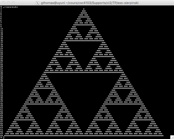
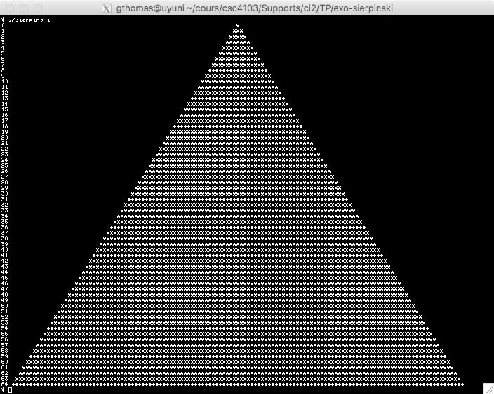
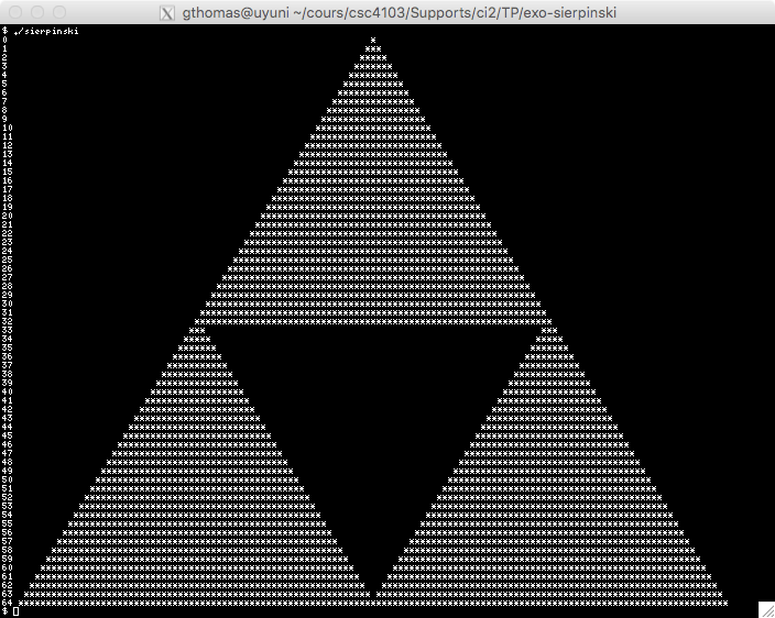
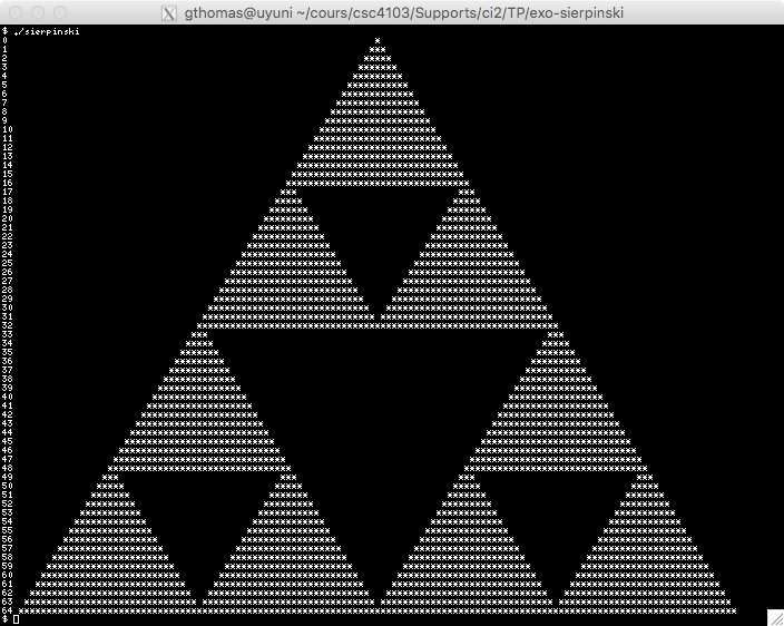
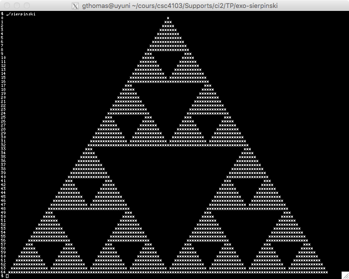
The goal of this exercise is to create an approximation of the Sierpinski triangle as shown in Figure .
 |
 |
 |
 |
| Step 0 | Step 1 | Step 2 | Step 3 |
In this exercise, we build the approximation of the triangle at step n. To do this, we use a slightly different algorithm, which involves directly drawing the 3n triangles.
To build the Sierpinski triangle, we will need to sort an array of floating-point numbers. In this first part, we will implement the sorting algorithm. We use the insertion sort algorithm. This algorithm is not very efficient for sorting large sequences but proves to be particularly effective on small sequences.
+-----------------------+
| 1 | 3 | 5 | 7 | | |
+-----------------------+
|
+-----------------------+
| 1 | 3 | 5 | 7 | | |
+-----------------------+
↑ |
+-----------------------+
| 1 | 3 | 5 | 7 | | |
+-----------------------+
↑ |
| a. Initial array | b. Searching for position for 4 | c. Finds position for 4 |
+-----------------------+
| 1 | 3 | 5 | 5 | 7 | |
+-----------------------+
↑ |
+-----------------------+
| 1 | 3 | 4 | 5 | 7 | |
+-----------------------+
↑ |
| d. Shifts right | e. Inserts 4 |
To begin, in the main function of sierpinski.c, declare an array named tab of floating-point numbers with 5 elements initialized to 1, 3, 5, 7, 0. Then, print the 5 elements of the array using a loop in the terminal.
We now implement the search function. Write a function sort_get_index taking as arguments:
- an array of floats named tab,
- the current maximum index of the array top minus one (in other words, this argument gives the number of elements already inserted in the array),
- a float to insert val.
This function assumes that only the elements from 0 to top-1 have been filled. It returns the index, between 0 and top, corresponding to the future position of the value val in the sorted array:
- The index, between 0 and top-1, containing the first value greater than val if it exists,
- The index top otherwise.
Test your function by displaying the insertion indices for the values 0, 3.5, and 10 using the array created in the previous question, where top is considered to be 4. Your program should produce an output similar to this:
We will now implement the function to shift right and insert. Write a function sort_insert_at taking as arguments:
- an array of floats named tab,
- the insertion index i,
- the current maximum index of the array top,
- the floating-point number to insert val.
This function should shift to the right the elements between i and top before placing val at position i. Note that you have to start by shifting the elements from the right of the array to avoid overwriting values.
Test your function by inserting the value 3.5 at index 2 before displaying your array in the main function. Your program should produce output similar to this:
We can now write the insertion function. Write a function named sort_insert taking the same arguments as sort_get_index. This function should use sort_get_index and sort_insert_at to insert the new element.
Test your function by replacing the test of sort_insert_at with the insertion of the element 2.
In this part, we create a finite grid. We represent a grid with n columns and m rows using a character array of size n * m. The first n elements contain the first row, the next n contain the second row, and so on.
To easily modify the size of our grid later, we define two functions named int nb_columns() and int nb_lines() which return the values 32 and 16, respectively. After removing the code that tests the sorting functions from the main function, display the dimensions of the grid in the main function to verify that your functions are correct.
In the main function, remove the display code, and instead create an array named grid of nb_lines() * nb_columns() characters. Set the first element of the grid to the value * and display this character.
Now that the grid is in place, we can initialize it. Write a function grid_init taking as arguments: (i) a character array grid and (ii) a character pixel. This function should initialize the nb_lines() * nb_columns() elements of the grid array to the value pixel.
In the main function, replace the initialization of the first character with the value * with initialization of the entire grid with the character *. Keep the display of the first element of the grid to verify that your program is correct.
The goal of this question is to write a function that displays the grid. Write a function grid_display taking as parameter a character array grid. This function should display, on each line of the terminal, a line of the grid.
In the main function, replace the display of the first element of the grid with the display of the entire grid.
Write a function named plot_point taking as parameters: (i) a grid grid, (ii) an integer coordinate x, (iii) an integer coordinate y, and (iv) a character pixel. This function should place the character pixel at position (x, y) in the grid.
In the exercise, we assume that the bottom-left corner of the grid corresponds to the point with coordinates (0, 0). Therefore, placing the character pixel at coordinates (x, y) means placing the character pixel at the intersection of row nb_lines() - y - 1 and column x.
To test your program, in the main function, place the space character (' ') at (3, 1), and carefully check that your coordinate system is oriented correctly.
You should obtain the following output:
To guard against potential bugs you might encounter, modify your plot_point function to display an error message and exit if x or y fall outside the grid. Verify that your code is correct by attempting to display the point with coordinates (3, 100).
To draw the Sierpinski triangle, you need to be able to draw filled polygons. And to draw filled polygons, you will need to draw vertical lines. Drawing a vertical line is not a major challenge, but the problem becomes slightly more complicated as the coordinates of the polygons will be represented by floating-point numbers. You need to be able to project a vertical line represented by floating-point coordinates onto a grid using integer coordinates.
Write a function plot_vline that takes as parameters :
- a character array grid,
- an integer x-coordinate x,
- a floating-point y-coordinate fy0,
- a floating-point y-coordinate fy1,
- a character pixel.
The function plot_vline should draw each of the points of the vertical line (x, fy0) to (x, fy1) in the grid using the character pixel. It is assumed that fy1 is greater than or equal to fy0 (this will be the case, as these y-coordinates will come from a sorted array).
As a first approximation, we suggest converting fy0 to an integer variable y0 and fy1 to an integer variable y1, then drawing each of the points on the x-axis that fall between y0 and y1 inclusive.
To test your program, start by initializing the grid with the space character (' ') instead of the '*' character. Then, draw the line from (1, 2) to (1, 3) using the character '|' with plot_vline. This program should draw a line including the points (1, 2) and (1, 3).
We are now dealing with correctly converting floating-point numbers to integers. Initially, we want to round the floating-point number to the nearest integer value. This way, the segment [1.2, 3.8] will be converted to [1, 4] and the segment [1.7, 3.3] to [2, 3]. This rounding provides a relatively aesthetic graphical result.
Unfortunately, converting a floating-point number to an integer in C simply truncates the decimal part of the floating-point number. Thus, currently, the number 3.8 is converted to 3, which is not what we expect. However, you may notice that if we round a floating-point number f by truncating the decimal part of f + 0.5, you get exactly the rounding we expect: 1.2 is converted to E(1.2 + 0.5) = 1 and 3.8 to E(3.8 + 0.5) = 4.
Modify your function plot_vline to perform this rounding. Test your rounding by drawing, after the line (1, 2) to (1, 3), the lines (2, 1.7) to (2, 3.3) and (3, 1.2) to (3, 3.8).
Now we face the problem of rounding numbers with a decimal part of exactly 0.5. Indeed, we could project the segment [0.5, 1.5] to [0, 2], [0, 1], [1, 2], or [1, 1]. All these solutions are correct, of course, but it is more aesthetic to restrict to symmetric projections around 1 : either [0, 2] or [1, 1]. With our current algorithm, the number 0.5 is converted to 1 and the number 1.5 to 2, which is not suitable. To adopt the first solution, we suggest subtracting 1 from y0 if fy0 is equal to y0 - 0.5, i.e., if the decimal part of fy0 is equal to 0.5.
Test your function by adding the line from (7, 0.5) to (7, 1.5) to your grid. The figure you should obtain at this stage is as follows :
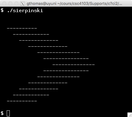
We can now start drawing the polygons that will be used to draw the Sierpinski triangle. The figure below presents the principle. A polygon is defined by a set of points called the vertices of the polygon. The goal of this part is to fill a polygon from its points. For example, the polygon represented in Figure is defined by the points (2, 13), (10, 13), (30, 7), (10, 1), (2, 1), (18, 7).
 |
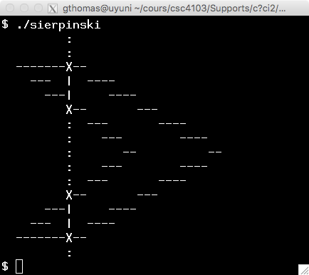 |
| a. The filled polygon | b. Sweeping the axis 9 |
To fill the polygon, we sweep the figure along the x-axis. Figure b represents the sweeping of axis 9. When sweeping an axis, we start by identifying all the intersections between the swept axis and the sides of the polygon. In our figure, by sweeping axis 9, we get the points (9, 1), (9, 3.625), (9, 10.375), and (9, 13) represented by the symbol X on the figure.
By sorting these points along the y-axis, we see that this sequence gives exactly the vertical lines to draw if we take the points two by two : in our case, it is enough to draw the lines (9, 1) to (9, 3.625) and (9, 10.325) to (9, 13).
We begin by setting up the definition of a polygon and the sweeping algorithm. For this, you need to :
- Define a structure named point containing two floating-point fields named x and y.
- Write a function named plot_poly_sweep that takes a grid, an array of points, the number of points in the array, the x-coordinate of the swept axis (an integer), and a pixel (a character). For now, this function should display the swept axis.
- Write a function named plot_poly that takes a grid, an array of points, the number of points in the array, and a pixel (a character). This function should iterate with a variable x over the values 0 to nb_columns() and call plot_poly_sweep for each swept axis.
- Remove from the main function the construction of the lines requested in the previous part, but keep the definition of the grid, its initialization, and its display.
- Create an array of points named p in the main function. This array should be initialized with the following points : { 2, 13 }, { 10, 13 }, { 30, 7 }, { 10, 1 }, { 2, 1 }, { 18, 7 } (be sure to copy/paste this line into your program).
- Call the plot_poly function from the main function, between the initialization and the display of the grid.
When you run your program, you should get an output similar to this :
In order to find the intersection points between the swept x-axis and the sides of the polygon, we will iterate over each side of the polygon in the plot_poly_sweep function. Technically, iterating over the sides of the polygon is equivalent to iterating over the set of pairs: (p[n-1], p[0]), (p[0], p[1]), (p[1], p[2]), ..., (p[n-2], p[n-1]), where n is the number of points of the polygon. In each iteration, the variable j should be the index of the left element of a pair and the variable i should be the index of the right element. In this question, we will only display these pairs (not their values: only their indexes). The output produced by your program should thus now be similar to this since our polygon has 5 vertices:
For each side of the polygon, we want to know if the x-axis crosses this side, and at which point:
- To check if the x-axis may cross the side, simply verify that x is between p[i].x and p[j].x or between p[j].x and p[i].x.
- To find the potential intersection point between a side and an x-axis, some basic geometry is required. If you take the time to set up the problem, you would find easily (we hope) that this intersection point is p[i].y + (x - p[i].x) * (p[j].y - p[i].y) / (p[j].x - p[i].x) since the slope of the line passing through p[i] and p[j] is (p[j].y - p[i].y) / (p[j].x - p[i].x).
Start by removing the display of the pairs in your loop. Then, for each swept x-axis, instead, display the potential intersection point between the side and the x-axis.
You should get an output similar to this:
The algorithm you just implemented is not yet completely correct because some points (the corners) appear multiple times. In some cases, they need to appear, in others, they should not (especially on axis 10). However, before fixing this issue, we will draw the vertical lines: it is much easier to reason and correct a drawing rather than a series of points.
Before we can draw our lines, they need to be sorted. For this, we will reuse the sort_insert function defined in the first step. Modify your plot_poly_sweep function to:
- Create an uninitialized array of n * 4 floats named vlines at the beginning of the function (where n is the number of points passed as a parameter to the function),
- Define a variable named top to keep track of how many points are currently in this array,
- Remove the display of the intersection point and replace it with adding the intersection point to the vlines array using the sort_insert function,
- Display the points in the array after the loop that iterates over each side. You should get the same display as before, but the pointsshould now be sorted.
We can now draw the polygon. After displaying the intersection points, draw the lines by pairing the points in the array. Typically, if the intersection points are { 1, 1.375, 12.625, 13 }, you need to display the vertical lines [1, 1.375] and [12.625, 13] on the x-axis. You may notice that your polygon is almost correct, except for axis 10, where some vertical lines are reversed:
We are now fixing the problem with axis 10. The issue is that points 1 and 13 appear twice instead of once. For example, for point 1, this phenomenon is due to the fact that axis 10 intersects the line from (30, 7) to (10, 1), but also the line from (10, 1) to (2, 1).
To count these points only once, you should cut the plane between [0, x] and ]x, nb_columns()]: if [p[i].x, p[j].x] cuts the right part of the plane, count the intersection; otherwise, ignore it. For the case of point 1, we will count the side from (30, 7) to (10, 1), but not the one from (2, 1) to (10, 1). This invariant can be reformulated as follows:
- If p[i].x <= p[j].x, then we consider an intersection if p[i].x <= x and x < p[j].x,
- If p[j].x <= p[i].x, then we consider an intersection if p[j].x <= x and x < p[i].x.
Noting that the "If" part of our invariant is implied by the "Then" part, correct your program. You should obtain the following result:
optional
Our polygon is almost correct. However, some corners are no longer drawn, particularly point (30, 7) since the sides associated with this point are to the left in the plane. Similarly, a vertical line to the right of the figure would no longer be drawn. This result is acceptable if the resolution is high. However, if you want to correct this problem, you can slightly enrich your algorithm by drawing the missing points and lines in the loop that iterates over the sides:
- If p[i].x is equal to x, then
- If p[j].x is equal to x, we are dealing with a vertical side. We draw this side directly using plot_vline. Remember to consider the case where p[i].y < p[j].y and the reverse case because plot_vline needs to receive the arguments fy1 and fy2 in the correct order.
- Otherwise, we are dealing with a corner. We draw the point directly using plot_vline to draw a line from p[i].y to p[i].y.
- Then, whether or not p[i].x is equal to x, we handle adding the intersection point as in the previous question.
Now that we can draw polygons, we can finally draw this Sierpinski triangle.
Write a plot_triangle function taking as parameters a grid, three points p1, p2, and p3 and a pixel. This function should display the filled triangle using plot_poly.
Remove the displays done in the plot_poly function. Also remove the old tests from your main function. Finally, modify the size of your grid to have 65 rows and 129 columns and draw a filled triangle with coordinates (0, 0), (64, 64), (128, 0).
Since you will need to find the midpoints of the sides of the Sierpinski triangles, write a function named line_middle taking as parameters two points and returning the point at the midpoint of the segment.
Finally, write a recursive sierpinski function taking as parameters a grid, three points, a number n of remaining iterations and a pixel. This function should display the triangle if n equals 1, otherwise, this function should call sierpinski three times with each of the remaining full triangles at step n-1. Test your function with 6 iterations. You should get the result given at the beginning of the exercise.
